Multiple Outputs

Multiple Outputs

You will build neural networks with multiple outputs in this chapter, which can be used to solve regression problems with multiple targets. Additionally, you will build a model that simultaneously solves a regression problem and a classification problem.

This Multiple Outputs is part of [Datacamp course: Advanced Deep Learning with Keras] You will learn how to use the versatile Keras functional API to solve a variety of problems. The course will begin with simple, multi-layer dense networks (also known as multi-layer perceptrons) and progress to more sophisticated architectures. This course will cover how to construct models with multiple inputs and a single output, as well as how to share weights between layers in a model. Additionally, we will discuss advanced topics such as category embeddings and multiple output networks. This course will teach you how to train a network that performs both classification and regression.

This is my learning experience of data science through DataCamp. These repository contributions are part of my learning journey through my graduate program masters of applied data sciences (MADS) at University Of Michigan, DeepLearning.AI, Coursera & DataCamp. You can find my similar articles & more stories at my medium & LinkedIn profile. I am available at kaggle & github blogs & github repos. Thank you for your motivation, support & valuable feedback.

These include projects, coursework & notebook which I learned through my data science journey. They are created for reproducible & future reference purpose only. All source code, slides or screenshot are intellactual property of respective content authors. If you find these contents beneficial, kindly consider learning subscription from DeepLearning.AI Subscription, Coursera, DataCamp

import tensorflow as tf
import numpy as np
import pandas as pd
import matplotlib.pyplot as plt

plt.rcParams['figure.figsize'] = (8, 8)

Two-output models

Simple two-output model

In this exercise, you will use the tournament data to build one model that makes two predictions: the scores of both teams in a given game. Your inputs will be the seed difference of the two teams, as well as the predicted score difference from the model you built in chapter 3.

The output from your model will be the predicted score for team 1 as well as team 2. This is called “multiple target regression”: one model making more than one prediction

from tensorflow.keras.layers import Input, Dense
from tensorflow.keras.models import Model

# Define the input
input_tensor = Input(shape=(2, ))

# Define the output
output_tensor = Dense(2)(input_tensor)

# Create a model
model = Model(input_tensor, output_tensor)

# Compile the model
model.compile(optimizer='adam', loss='mean_absolute_error')

Metal device set to: Apple M2 Pro

Fit a model with two outputs

Now that you’ve defined your 2-output model, fit it to the tournament data. I’ve split the data into games_tourney_train and games_tourney_test, so use the training set to fit for now.

This model will use the pre-tournament seeds, as well as your pre-tournament predictions from the regular season model you built previously in this course.

As a reminder, this model will predict the scores of both teams.

games_tourney = pd.read_csv('dataset/games_tourney.csv')
games_tourney.head()

	season	team_1	team_2	home	seed_diff	score_diff	score_1	score_2	won
0	1985	288	73	0	-3	-9	41	50	0
1	1985	5929	73	0	4	6	61	55	1
2	1985	9884	73	0	5	-4	59	63	0
3	1985	73	288	0	3	9	50	41	1
4	1985	3920	410	0	1	-9	54	63	0

games_season = pd.read_csv('dataset/games_season.csv')
games_season.head()

	season	team_1	team_2	home	score_diff	score_1	score_2	won
0	1985	3745	6664	0	17	81	64	1
1	1985	126	7493	1	7	77	70	1
2	1985	288	3593	1	7	63	56	1
3	1985	1846	9881	1	16	70	54	1
4	1985	2675	10298	1	12	86	74	1

from tensorflow.keras.layers import Embedding, Input, Flatten, Concatenate, Dense
from tensorflow.keras.models import Model

# Count the unique number of teams
n_teams = np.unique(games_season['team_1']).shape[0]

# Create an embedding layer
team_lookup = Embedding(input_dim=n_teams,
                        output_dim=1,
                        input_length=1,
                        name='Team-Strength')

# Create an input layer for the team ID
teamid_in = Input(shape=(1, ))

# Lookup the input in the team strength embedding layer
strength_lookup = team_lookup(teamid_in)

# Flatten the output
strength_lookup_flat = Flatten()(strength_lookup)

# Combine the operations into a single, re-usable model
team_strength_model = Model(teamid_in, strength_lookup_flat, name='Team-Strength-Model')

# Create an Input for each team
team_in_1 = Input(shape=(1, ), name='Team-1-In')
team_in_2 = Input(shape=(1, ), name='Team-2-In')

# Create an input for home vs away
home_in = Input(shape=(1, ), name='Home-In')

# Lookup the team inputs in the team strength model
team_1_strength = team_strength_model(team_in_1)
team_2_strength = team_strength_model(team_in_2)

# Combine the team strengths with the home input using a Concatenate layer,
# then add a Dense layer

out = Concatenate()([team_1_strength, team_2_strength, home_in])
out = Dense(1)(out)

# Make a model
p_model = Model([team_in_1, team_in_2, home_in], out)

# Compile the model
p_model.compile(optimizer='adam', loss='mean_absolute_error')

# Fit the model to the games_season dataset
p_model.fit([games_season['team_1'], games_season['team_2'], games_season['home']],
          games_season['score_diff'],
          epochs=1, verbose=True, validation_split=0.1, batch_size=2048)

games_tourney['pred'] = p_model.predict([games_tourney['team_1'],
                                       games_tourney['team_2'],
                                       games_tourney['home']])

2023-04-08 01:04:42.790937: W tensorflow/tsl/platform/profile_utils/cpu_utils.cc:128] Failed to get CPU frequency: 0 Hz

138/138 [==============================] - 3s 11ms/step - loss: 12.2298 - val_loss: 11.6713
133/133 [==============================] - 0s 2ms/step

games_tourney_train = games_tourney[games_tourney['season'] <= 2010]
games_tourney_test = games_tourney[games_tourney['season'] > 2010]

model.fit(games_tourney_train[['seed_diff', 'pred']],
          games_tourney_train[['score_1', 'score_2']],
          verbose=False,
          epochs=10000,
          batch_size=256);

Inspect the model (I)

Now that you’ve fit your model, let’s take a look at it. You can use the .get_weights() method to inspect your model’s weights.

The input layer will have 4 weights: 2 for each input times 2 for each output.

The output layer will have 2 weights, one for each output.

# Print the model's weights
print(model.get_weights())

# Print the column means of the training data
print(games_tourney_train.mean())

[array([[ 0.57821244, -0.66847074],
       [23.578228  , 21.29037   ]], dtype=float32), array([67.67261, 68.08015], dtype=float32)]
season        1997.548544
team_1        5560.890777
team_2        5560.890777
home             0.000000
seed_diff        0.000000
score_diff       0.000000
score_1         71.786711
score_2         71.786711
won              0.500000
pred             0.141091
dtype: float64

Evaluate the model

Now that you’ve fit your model and inspected it’s weights to make sure it makes sense, evaluate it on the tournament test set to see how well it performs on new data.

print(model.evaluate(games_tourney_test[['seed_diff', 'pred']],
                     games_tourney_test[['score_1', 'score_2']],
                     verbose=False))

8.862776756286621

Single model for classification and regression

Classification and regression in one model

Now you will create a different kind of 2-output model. This time, you will predict the score difference, instead of both team’s scores and then you will predict the probability that team 1 won the game. This is a pretty cool model: it is going to do both classification and regression!

In this model, turn off the bias, or intercept for each layer. Your inputs (seed difference and predicted score difference) have a mean of very close to zero, and your outputs both have means that are close to zero, so your model shouldn’t need the bias term to fit the data well.

input_tensor = Input(shape=(2, ))

# Create the first output
output_tensor_1 = Dense(1, activation='linear', use_bias=False)(input_tensor)

# Create the second output(use the first output as input here)
output_tensor_2 = Dense(1, activation='sigmoid', use_bias=False)(output_tensor_1)

# Create a model with 2 outputs
model = Model(input_tensor, [output_tensor_1, output_tensor_2])

from tensorflow.keras.utils import plot_model

plot_model(model, to_file='Images/multi_output_model.png')

data = plt.imread('Images/multi_output_model.png')
plt.imshow(data);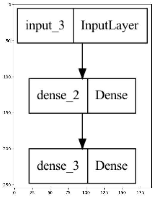

Compile and fit the model

Now that you have a model with 2 outputs, compile it with 2 loss functions: mean absolute error (MAE) for ‘score_diff’ and binary cross-entropy (also known as logloss) for ‘won’. Then fit the model with ‘seed_diff’ and ‘pred’ as inputs. For outputs, predict ‘score_diff’ and ‘won’.

This model can use the scores of the games to make sure that close games (small score diff) have lower win probabilities than blowouts (large score diff).

The regression problem is easier than the classification problem because MAE punishes the model less for a loss due to random chance. For example, if score_diff is -1 and won is 0, that means team_1 had some bad luck and lost by a single free throw. The data for the easy problem helps the model find a solution to the hard problem.

from tensorflow.keras.optimizers import Adam

# Compile the model with 2 losses and the Adam optimizer with a higher learning rate
model.compile(loss=['mean_absolute_error', 'binary_crossentropy'], optimizer=Adam(lr=0.01))

# Fit the model to the tournament training data, with 2 inputs and 2 outputs
model.fit(games_tourney_train[['seed_diff', 'pred']],
          [games_tourney_train[['score_diff']], games_tourney_train[['won']]],
          epochs=20,
          verbose=True,
          batch_size=16384);

WARNING:absl:At this time, the v2.11+ optimizer `tf.keras.optimizers.Adam` runs slowly on M1/M2 Macs, please use the legacy Keras optimizer instead, located at `tf.keras.optimizers.legacy.Adam`.
WARNING:absl:`lr` is deprecated in Keras optimizer, please use `learning_rate` or use the legacy optimizer, e.g.,tf.keras.optimizers.legacy.Adam.
WARNING:absl:There is a known slowdown when using v2.11+ Keras optimizers on M1/M2 Macs. Falling back to the legacy Keras optimizer, i.e., `tf.keras.optimizers.legacy.Adam`.

Epoch 1/20
1/1 [==============================] - 1s 832ms/step - loss: 11.3476 - dense_2_loss: 10.6665 - dense_3_loss: 0.6811
Epoch 2/20
1/1 [==============================] - 0s 13ms/step - loss: 11.3453 - dense_2_loss: 10.6633 - dense_3_loss: 0.6820
Epoch 3/20
1/1 [==============================] - 0s 12ms/step - loss: 11.3429 - dense_2_loss: 10.6601 - dense_3_loss: 0.6828
Epoch 4/20
1/1 [==============================] - 0s 12ms/step - loss: 11.3406 - dense_2_loss: 10.6569 - dense_3_loss: 0.6837
Epoch 5/20
1/1 [==============================] - 0s 11ms/step - loss: 11.3382 - dense_2_loss: 10.6537 - dense_3_loss: 0.6846
Epoch 6/20
1/1 [==============================] - 0s 10ms/step - loss: 11.3359 - dense_2_loss: 10.6504 - dense_3_loss: 0.6855
Epoch 7/20
1/1 [==============================] - 0s 9ms/step - loss: 11.3336 - dense_2_loss: 10.6472 - dense_3_loss: 0.6863
Epoch 8/20
1/1 [==============================] - 0s 12ms/step - loss: 11.3312 - dense_2_loss: 10.6440 - dense_3_loss: 0.6872
Epoch 9/20
1/1 [==============================] - 0s 9ms/step - loss: 11.3289 - dense_2_loss: 10.6408 - dense_3_loss: 0.6881
Epoch 10/20
1/1 [==============================] - 0s 9ms/step - loss: 11.3266 - dense_2_loss: 10.6376 - dense_3_loss: 0.6890
Epoch 11/20
1/1 [==============================] - 0s 10ms/step - loss: 11.3243 - dense_2_loss: 10.6344 - dense_3_loss: 0.6898
Epoch 12/20
1/1 [==============================] - 0s 9ms/step - loss: 11.3219 - dense_2_loss: 10.6312 - dense_3_loss: 0.6907
Epoch 13/20
1/1 [==============================] - 0s 9ms/step - loss: 11.3196 - dense_2_loss: 10.6280 - dense_3_loss: 0.6916
Epoch 14/20
1/1 [==============================] - 0s 9ms/step - loss: 11.3173 - dense_2_loss: 10.6248 - dense_3_loss: 0.6924
Epoch 15/20
1/1 [==============================] - 0s 8ms/step - loss: 11.3150 - dense_2_loss: 10.6216 - dense_3_loss: 0.6933
Epoch 16/20
1/1 [==============================] - 0s 9ms/step - loss: 11.3126 - dense_2_loss: 10.6184 - dense_3_loss: 0.6942
Epoch 17/20
1/1 [==============================] - 0s 9ms/step - loss: 11.3103 - dense_2_loss: 10.6152 - dense_3_loss: 0.6951
Epoch 18/20
1/1 [==============================] - 0s 9ms/step - loss: 11.3080 - dense_2_loss: 10.6121 - dense_3_loss: 0.6959
Epoch 19/20
1/1 [==============================] - 0s 17ms/step - loss: 11.3056 - dense_2_loss: 10.6089 - dense_3_loss: 0.6968
Epoch 20/20
1/1 [==============================] - 0s 9ms/step - loss: 11.3033 - dense_2_loss: 10.6057 - dense_3_loss: 0.6977

Inspect the model (II)

Now you should take a look at the weights for this model. In particular, note the last weight of the model. This weight converts the predicted score difference to a predicted win probability. If you multiply the predicted score difference by the last weight of the model and then apply the sigmoid function, you get the win probability of the game.

# Print the model weights
print(model.get_weights())

# Print the training data means
print(games_tourney_train.mean())

[array([[ 0.33446303],
       [-1.1826252 ]], dtype=float32), array([[1.3517005]], dtype=float32)]
season        1997.548544
team_1        5560.890777
team_2        5560.890777
home             0.000000
seed_diff        0.000000
score_diff       0.000000
score_1         71.786711
score_2         71.786711
won              0.500000
pred             0.141091
dtype: float64

from scipy.special import expit as sigmoid

# Weight from the model
weight=0.14

# Print the approximate win probability predicted close game
print(sigmoid(1 * weight))

# Print the approximate win probability predicted blowout game
print(sigmoid(10 * weight))

0.5349429451582145
0.8021838885585818

Evaluate on new data with two metrics

Now that you’ve fit your model and inspected its weights to make sure they make sense, evaluate your model on the tournament test set to see how well it does on new data.

Note that in this case, Keras will return 3 numbers: the first number will be the sum of both the loss functions, and then the next 2 numbers will be the loss functions you used when defining the model.

print(model.evaluate(games_tourney_test[['seed_diff', 'pred']],
                    [games_tourney_test[['score_diff']], games_tourney_test[['won']]],
                     verbose=False))

[11.036083221435547, 10.24341106414795, 0.7926721572875977]